Boxing Pythagoras

Infinitesimal Calculus 2: The Changes in Change

The mathematics of change are quite interesting. In a naive sense, we can often describe a change by a simple collection of data points. For example, let’s think about a little boy rolling a ball across the floor. The boy pushes the ball, and four seconds later, the ball has come to be 2 meters away from him. Given these data points, we may attempt to connect them in some meaningful analytical manner– perhaps by saying that the ball rolled at a speed of half a meter per second. But even this is a somewhat naive bit of information, as it only really tells us something about the completed journey. Mathematicians are greedy, however; they want to be able to know about every point of the ball’s travel, at any arbitrary moment in time.

We can use a function for just such a purpose. A function is a specific mathematical tool which allows us to describe an entire set of data points all at once which we symbolize as (read “ of “). We encode the data by means of a mathematical formula. For example, our exemplary rolling ball might well have been encoded by the function , where the represents the time, in seconds, that the ball has been rolling, and the value of the function, tells us the distance in meters which the ball has traveled in that time. In this particular function, the coefficient of tells us the rate at which distance changes as time passes– that is, a meter per second. When the boy first rolls it, the ball is traveling at a meter per second; when it finishes it had been traveling at a meter per second; and at any single point during the journey the ball is traveling at a meter per second.

However, this is a very simple example. It describes a situation involving a constant velocity. Things become a bit more muddied when the rate at which a change occurs is, itself, changing.

Our example above describes a linear function. Linear functions are so named because they can be graphed on a Cartesian plane to form a straight line. The equation for a linear function is of the form , where represents the y-intercept (the point at which the line crosses over the y-axis of the plane) and where represents the slope of the line (the rate of change for the function). Utilizing the function from our example, , we have a slope of , an intercept of 0, and we can produce the following graph:

Figure 1: Graph of a Linear Function

It’s very easy to see, intuitively, that this line’s slope, or rate of change, is constant throughout the whole function. We don’t even need to see the equation which generated this graph to see that this is the case, if we presume that the line on the graph is actually as straight as it appears. That very straightness is precisely what we mean by a constant rate of change. As such, it is perfectly clear that the graph has the same slope at as it does at or or . Regardless of how far along the graph we look, it will always have the same rate of change.

However, this is not true of all graphs. When a function ceases to be linear, the rate of change of that function ceases to be constant. Take, for example, the following graph of the function :

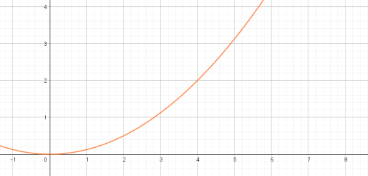
Figure 2: Graph of a Parabolic Function

Let’s pretend that, instead of rolling the ball across a flat floor, the little boy has instead set the ball atop a ramp and let go. The ball starts moving slowly, but builds up more and more speed as it moves farther and farther from the boy.  After four seconds, the ball is two meters away from the boy– just as in our first example– which means that the ball still traveled a meter per second, overall. However, it seems entirely clear that the ball was not moving at that speed at every single moment in the journey, the way it had when the boy rolled it across the floor. At the start of its roll, the ball is moving much slower than  a meter per second, while at the end it is moving much faster than  a meter per second.

This introduces a very interesting, and very important, question: how can we tell what the rate of change is at any given point? What is the instantaneous rate of change?

For example, let’s say I want to know how fast the ball is moving precisely 3 seconds after the boy has set it rolling. A person might think that they can simply determine how far the ball has gone in that time– meters– and then divide that distance by the time– 3 seconds– to conclude that the ball is traveling at  of a meter per second. However, this has the same problem as the whole 4 second journey: the ball seems to be traveling slower than  of a meter per second at the start and faster than of a meter per second toward the end.

One way in which we know this fact is by looking at how far the ball travels between the second and third seconds of its journey. So, after two seconds, the ball is a meter from its starting point. After three seconds, it is of a meter from the starting point. This indicates that the ball traveled of a meter in one second. But this, again, falls prey to the same problem we’ve been having: the ball seems to be moving more slowly than of a meter per second at the 2 second mark and more swiftly at the 3 second mark. We’re closer to the speed of the ball at 3 seconds than we were before, but we still haven’t determined it, quite yet.

We can continue to take smaller intervals of time in order to find better and better approximations of the speed of the ball at the 3 second mark. For example, using the distance the ball moves between the 2.5 second and 3 second marks, or the 2.75 second and 3 second marks, or the 2.99999999998 second and 3 second marks. We can come really, really close to the answer we’re trying to find by doing this, but we don’t end up with the exact answer– and mathematicians are not happy to settle for an inexact answer.

Let’s think about what we are doing in these approximations.

Figure 3: Approximating the Speed at 3 Seconds

If the ball had traveled at a constant speed from the start, at time 0, to the 3 second mark, then its journey could be represented with line . The slope of this line is — which is the approximate speed we determined when considering the ball over this period. Similarly, the line has a slope of , our approximation from the 2 second mark to the 3 second mark. If we were to calculate the slope of , our approximation would get even better. Visually, in the graph above, we can see that the linear graphs are getting closer and closer to the parabolic graph– but there’s always some tiny bit of space between the two.

Algebraically speaking, what are we doing in these approximations? How can we translate this problem into our mathematical language?

Well, we are taking the distance which the ball has traveled after 3 seconds– which, in our math language, is — and we are subtracting the distance which the ball had traveled at an earlier time– say, or or — to find the distance which the ball has traveled between those two times. We are then dividing this distance by the amount of time which has elapsed between the two points: seconds or second or seconds.

Now let’s try to generalize this. We have our function, . We are looking at the difference between the value of the function at some point, , and the value of the function at some subsequent point, ; we are then dividing that difference by the difference in our two points, — which is just . So, this leads us to the expression .

As we have seen, the smaller the gap between our two -values, the closer our approximation becomes. Naturally, we might then think that we can find an exact solution to our problem if we just remove the gap, entirely– that is to say, what happens if we set equal to zero in the expression that we found, above? However, we very quickly come to a problem if we do that. Evaluating the expression, we’ll see that . This is certainly problematic– any middle school child should be able to point out that we simply cannot evaluate that .

But what if we had some number which wasn’t zero, and yet that number was infinitely close to ? In such a case, we could reasonably assume that our answer is infinitely close to being correct.

Thankfully, in the first part of this series, we learned that we do have such numbers: the infinitesimals. So now, if I replace the from our above expression with any arbitrary infinitesimal– let’s call it — we’ll find that evaluates to something infinitely close to the answer which we are looking to find. For the exact answer, as we mentioned, we would like to have been able to replace the with zero; but now we can be clever. Instead of trying to do undefined operations of math, dividing zero by zero, we can find the Real number solution which is infinitely close to our evaluated expression, which (as you will recall) is called the standard part of the expression. By taking the standard part of , we can find the exact answer to our problem.

Let’s go back to our rolling ball, now, to see how we can put this into use. We want to find the exact speed of the ball at the 3 second mark. Translating this into our expression, we get:

So, precisely at the 3 second mark, we now know that the ball is traveling at exactly of a meter per second. However, we can do even better than this. As mentioned earlier, mathematicians are greedy. We don’t just want to know what’s going on at a few of the points; we want to know what is going on at all of the points. So, rather than solving for some particular value of , such as 3, we can solve the expression for all values of , like so:

This new function, , is called the derivative of our original function. We denote the derivative of with an apostrophe, written as and often read as “-prime of .”

The derivative is a very powerful tool. It gives us a way of describing the instantaneous rate of change for all points of a given function. When discussing speed or velocity, as we have been doing for our exemplary ball, the derivative of the function for distance gives a function describing velocity. The derivative of the function describing velocity will, in turn, give us a function describing acceleration. Taking the derivative of that function will then tell us how quickly our acceleration is, itself, increasing or decreasing– and so on and so forth. When we take derivatives of derivatives, like this, we refer to them as second, third, fourth derivatives (and so on). So, as we have now seen, the second derivative of a distance function is an acceleration function.

The derivative was developed by mathematicians for the express purpose of describing the changes in change. By its use and exploration, we can conquer a great many problems which are incredibly difficult– or even impossible– without this wonderful tool. And, at the very heart of the derivative lie the infinitesimals– these numbers between our numbers– which give this mathematical tool its power.